EnergyPlus Shadow Calculation Inputs
Analysis description
As part of my work providing Building Energy Modeling Services to MapMortar, I encountered a pratical challenge: adding surrounding buildings to a model let to a dramatic increase in EnergyPlus simulation time: from 8s to 2min30s. This was not acceptable for MapMortar, so we decided to investigate how to maintain modelling accuracy while keeping calculation times under control.
For MapMortar, modelling accuracy and spatial context are both essential. Energy performance is strongly influenced by the surrounding built environment, and omitting nearby buildings would have compromised the validity of the results. At the same time, the approach had to remain computationally viable when applied across large portfolios.
Note: This post showcases analysis carried out on a single large model. The final technical solution implemented by MapMortar did not rely solely on tuning EnergyPlus input parameters, but on the development of an algorithm to pre-process surrounding-building geometry and remove shading surfaces that do not materially affect results
You can learn more about ![]() at https://www.mapmortar.io/
at https://www.mapmortar.io/
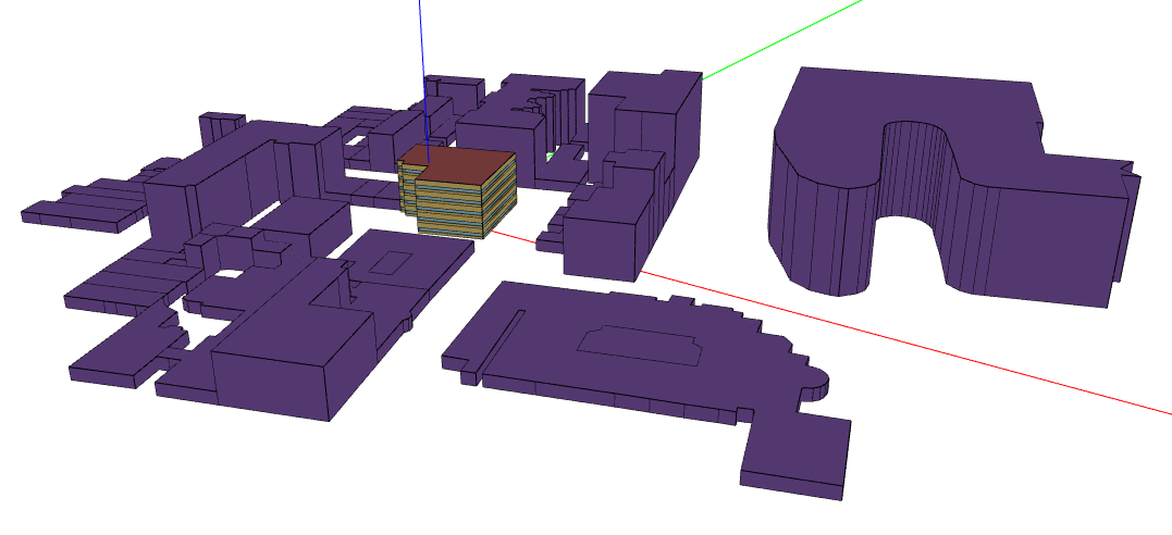
The surrounding buildings were added greedily by querying GIS data and constructing the geometry, not manually. As such a lot of shading surfaces were created, and some of which would never cast a shadow because there were closer surfaces that would also shade. The resulting shading geometry contained 61 ShadingSurfaceGroups (=surrounding buildings) for a total of 707 ShadingSurfaces.
The Total Site Energy Usage (GJ) for a year run:
- No shading: 2748.45 GJ
- With Shading: 2732.07 GJ
At that point in time, the ShadowCalculation object is purely defaulted:
ShadowCalculation,
  PolygonClipping,                        !- Shading Calculation Method
  Periodic,                               !- Shading Calculation Update Frequency Method
  20,                                     !- Shading Calculation Update Frequency
  15000,                                  !- Maximum Figures in Shadow Overlap Calculations
  SutherlandHodgman,                      !- Polygon Clipping Algorithm
  512,                                    !- Pixel Counting Resolution
  SimpleSkyDiffuseModeling,               !- Sky Diffuse Modeling Algorithm
  No,                                     !- Output External Shading Calculation Results
  No,                                     !- Disable Self-Shading Within Shading Zone Groups
  No;                                     !- Disable Self-Shading From Shading Zone Groups to Other Zones
In the Object Building, the Field Solar Distribution == FullExterior, and that will not change throughout this analysis.
Initial investigation
Removing the useless roofs
First off, the eplusout.err would indicate that some surfaces were non-convex:
   ** Warning ** DetermineShadowingCombinations: There are 39 surfaces which are receiving surfaces and are non-convex.
   **   ~~~   ** ...Shadowing values may be inaccurate. Check .shd report file for more surface shading details
   **   ~~~   ** ...Add Output:Diagnostics,DisplayExtraWarnings; to see individual warnings for each surface.
As can be seen visually on the above image, the surrounding building roofs are:
- Non-convex
- And useless from a shading perspective, because the assumption in creating the surrounding buildings was to take a flat roof, so any ray coming from the sun, hitting the roof of the surrounding building and any surface on the receiving building of interest, would also hit one of the surrounding building’s wall.
So I started by not creating the roofs anymore, which reduced the runtime down to 1min30s, so already a 1minute / 40% gain.
Using Pixel Counting (GPU)
I do have a GPU (a NVIDIA GeForce GTX 1060 6GB) on this machine, and given the large number of surfaces the overhead of moving data from the CPU to the GPU is well worth it. The I/O reference guide does mention that the tipping point where GPU makes sense is when you have more than 200 shading surfaces and I was well above that.
The runtime would decrease to a mere 13s, and the total site energy usage was 2729.16 GJ, a 0.1% difference with the default PolygonClipping Algorithm.
Unfortunately, for the underlying use case (running a server), this wasn’t an option.
Saving and reusing Shading Calculations
The underlying use case entails running a baseline, and dozen of ECMs, none of which would modify the geometry of the buildings, so saving the shading calculations when running the baseline and reusing them for all proposed runs could be a good option.
- When generating the results, via
Output External Shading Calculation Results=Yes, the runtime increases to 1min42s, so an overhead of 13s. - That creates a 512 MB
eplusshading.csvfile, which isn’t small. - Test with Algorithm =
Importedand aSchedule:File:Shadingobject: runtime is 28s, energy usage 2729.69 GJ (not sure why there’s a small diff there, maybe it’s because I kept the Shading Calculation Update Frequency as 20)
This would be a very valid option, but a couple of things push me to investigate more:
- The 512 MB is a problem for the cheaper server instances
- The OpenStudio SDK doesn’t support the
Schedule:File:Shadingobject (I opened NatLabRockies/OpenStudio#5600 to track it), so that’s going to require an OpenStudioEnergyPlusMeasure(which would be easy for me to write, but I’d have to be careful about moving the file around or passing absolute paths etc)
Parametric Analysis of the impact of the different ShadowCalculation parameters
Assuming the PixelCounting (GPU) is out of the question, and the saving/reusing is too, that leaves the different parameters of the PolygonClipping algorithm.
We’ll start with a base case (which is equivalent to the IDF Snippet given above):
def original(sc: ShadowCalculation) -> None:
    sc.setPolygonClippingAlgorithm("SutherlandHodgman")
    sc.setShadingCalculationUpdateFrequency(20)
    sc.setMaximumFiguresInShadowOverlapCalculations(15000)
    sc.setPixelCountingResolution(512)
From this default one/original, I’ll be testing varying one field at a time.
In each list below, the first element is the default one.
And I’ll be collecting E+ runtime in seconds AND Total Site Energy (GJ). Everything is done in Python.
# Polygon Clipping Algorithm
CLIPPING_ALGORITHMS = ["SutherlandHodgman", "ConvexWeilerAtherton", "SlaterBarskyandSutherlandHodgman"]

# Update Frequency
UPDATE_FREQUENCY = [20, 1, 31]

# Max Figures
MAX_FIGURES = [15_000, 200, 1_000, 5_000, 10_000]

# Pixel Counting Resolution
PIXEL_COUNTING_RESOLUTIONS = [512, 16, 64, 128, 256]
| test_name | Algorithm | Update Frequency | Max Figures | Pixel Resolution |
|---|---|---|---|---|
| original | SutherlandHodgman | 20 | 15000 | 512 |
| weiler | ConvexWeilerAtherton | 20 | 15000 | 512 |
| slater | SlaterBarskyandSutherlandHodgman | 20 | 15000 | 512 |
| update_frequency_31 | SutherlandHodgman | 31 | 15000 | 512 |
| max_figures_200 | SutherlandHodgman | 20 | 200 | 512 |
| max_figures_1000 | SutherlandHodgman | 20 | 1000 | 512 |
| max_figures_5000 | SutherlandHodgman | 20 | 5000 | 512 |
| max_figures_10000 | SutherlandHodgman | 20 | 10000 | 512 |
| pixel_counting_resolution_16 | SutherlandHodgman | 20 | 15000 | 16 |
| pixel_counting_resolution_64 | SutherlandHodgman | 20 | 15000 | 64 |
| pixel_counting_resolution_128 | SutherlandHodgman | 20 | 15000 | 128 |
| pixel_counting_resolution_256 | SutherlandHodgman | 20 | 15000 | 256 |
| minimal_everything | SutherlandHodgman | 31 | 200 | 16 |
Note: I’m not going to include the test case with Update Frequency = 1 day below, because it took 34min (!!) to run, but this is a nice reference point to know.
| Input | Absolute | Absolute difference | Relative difference | |||||||
|---|---|---|---|---|---|---|---|---|---|---|
| Algorithm | Update Frequency | Max Figures | Pixel Resolution | seconds | GJ | seconds | GJ | seconds | GJ | |
| test_name | ||||||||||
| original | SutherlandHodgman | 20 | 15000 | 512 | 94.14 | 2732.07 | 0.00 | 0.00 | 0.00% | 0.00% |
| weiler | ConvexWeilerAtherton | 20 | 15000 | 512 | 126.91 | 2727.54 | 32.77 | -4.53 | 34.81% | -0.17% |
| slater | SlaterBarskyandSutherlandHodgman | 20 | 15000 | 512 | 91.83 | 2732.22 | -2.30 | 0.15 | -2.45% | 0.01% |
| update_frequency_31 | SutherlandHodgman | 31 | 15000 | 512 | 63.29 | 2732.67 | -30.85 | 0.60 | -32.77% | 0.02% |
| max_figures_200 | SutherlandHodgman | 20 | 200 | 512 | 43.68 | 2729.73 | -50.45 | -2.34 | -53.59% | -0.09% |
| max_figures_1000 | SutherlandHodgman | 20 | 1000 | 512 | 50.05 | 2730.06 | -44.09 | -2.01 | -46.84% | -0.07% |
| max_figures_5000 | SutherlandHodgman | 20 | 5000 | 512 | 66.93 | 2731.41 | -27.20 | -0.66 | -28.90% | -0.02% |
| max_figures_10000 | SutherlandHodgman | 20 | 10000 | 512 | 81.12 | 2732.10 | -13.02 | 0.03 | -13.83% | 0.00% |
| pixel_counting_resolution_16 | SutherlandHodgman | 20 | 15000 | 16 | 94.01 | 2732.07 | -0.13 | 0.00 | -0.13% | 0.00% |
| pixel_counting_resolution_64 | SutherlandHodgman | 20 | 15000 | 64 | 93.64 | 2732.07 | -0.50 | 0.00 | -0.53% | 0.00% |
| pixel_counting_resolution_128 | SutherlandHodgman | 20 | 15000 | 128 | 92.33 | 2732.07 | -1.81 | 0.00 | -1.92% | 0.00% |
| pixel_counting_resolution_256 | SutherlandHodgman | 20 | 15000 | 256 | 94.06 | 2732.07 | -0.08 | 0.00 | -0.08% | 0.00% |
| minimal_everything | SutherlandHodgman | 31 | 200 | 16 | 32.92 | 2729.36 | -61.21 | -2.71 | -65.03% | -0.10% |
Interactive Parallel Coordinates Plot using d3.js
The plot is brushable.